Conics

An algebraic curve of degree 2 is a curve with an implicit equation given by a₁x²+2bxy+a₂y²+2c₁x+2c₂y+d=0, for given real numbers a₁, a₂, b, c₁, c₂ and d, and is called a conic. Indeed, since the theorems of the Belgian mathematicians Quetelet and Dandelin published in 1822, we know that an algebraic curve of degree 2 is always the intersection of a cone of revolution with a plane. Depending on the position of the plane according to the cone, one gets an ellipse, a hyperbola or a parabola. This is illustrated in the following images.

An ellipse: the angle between the plane and the axis of revolution is greater than the angle between the rulers and the axis of revolution.

A hyperbola: the angle between the plane and the axis of revolution is smaller than the angle between the rulers and the axis of revolution.

A parabola: the angle between the plane and the axis of revolution is equal to the angle between the rulers and the axis of revolution. The plane is in this case parallel to one of the rulers.

By making the right choice of orthonormal frame, the general equation of the non-degenerate conic can be simplified to one of the classical reduced equations. VisuMath will calculate the general equation of the conic and make a drawing of it in which all relevant axes are also drawn. First, one chooses the right type of conic and enters the appropriate values for the parameters.

Then the orthogonal transformation is entered. The orthogonal transformation, this is a rotation possible combined with a reflection, transforms the (X,Y)-axes to (X',Y')-axes. This transformation is entered by giving the images of the base vectors (up to a factor). Make sure that the vectors are orthogonal since we need an orthonormal frame. VisuMath will then norm these vectors (= rescale to length 1).

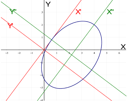
Then one needs to enter the translation that needs to be applied to the transformed frame (X',Y'). One obtains the new orthonormal frame (X",Y") with respect to which the conic has the simple reduced equation entered earlier. The translation is entered by giving the coordinates of the origin of the new orthonormal frame (X",Y") with respect to the frame (X',Y').

By hitting the button "Go", the general equation of the conic appears in its most simple form. Below, one finds the graph of an ellipse: